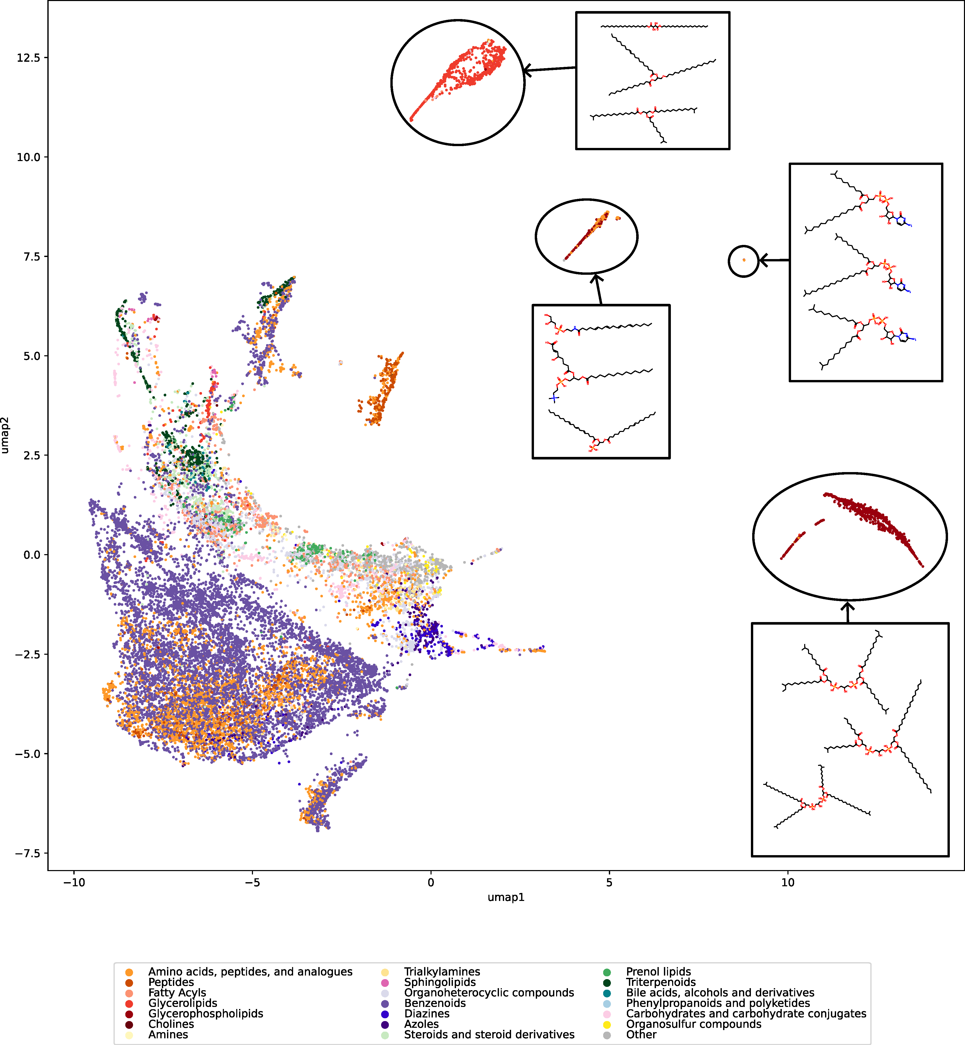
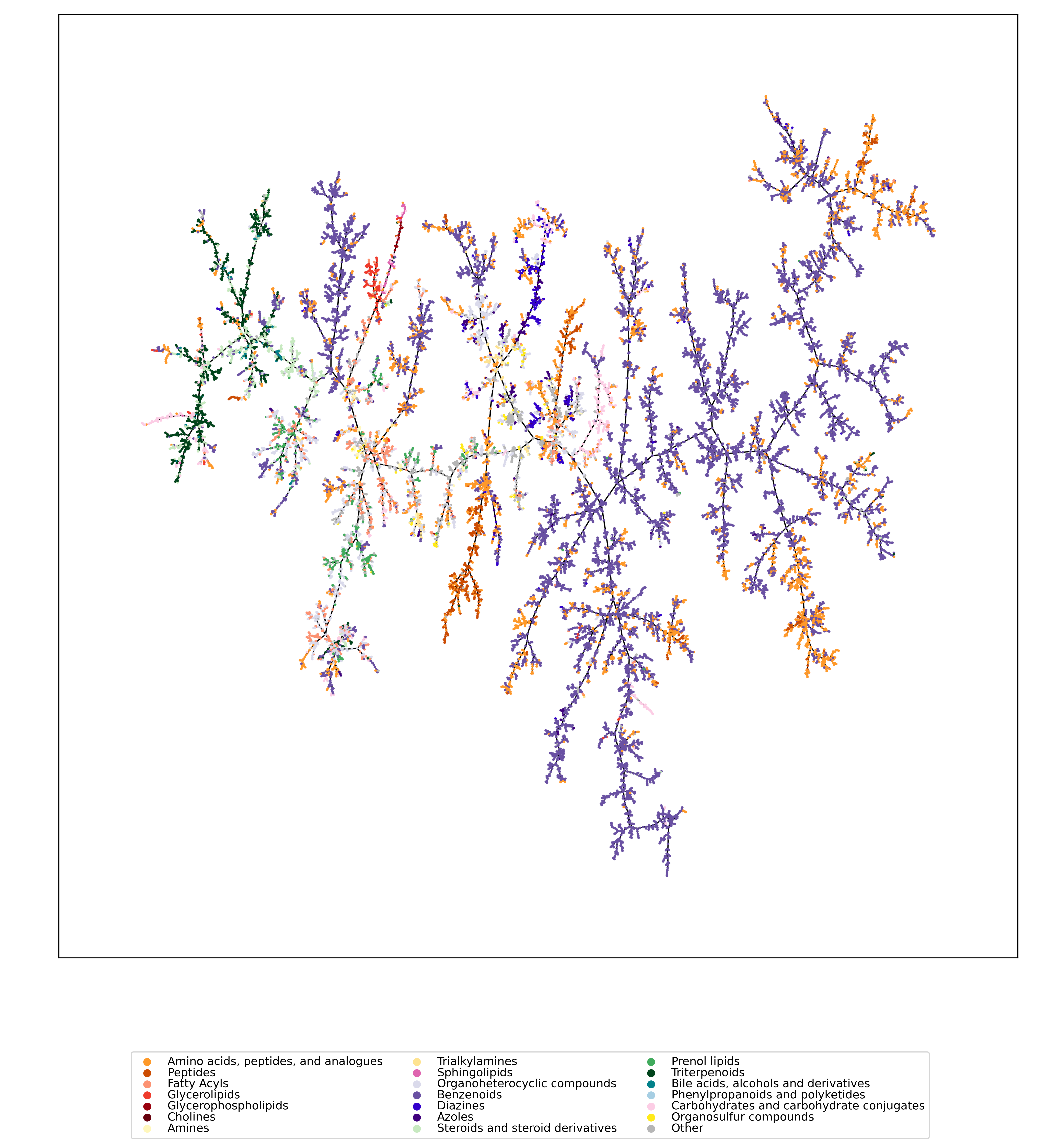
Have you ever wanted to look at the universe of biomolecules (small molecules of biological interest, including metabolites and toxins)? Have you ever wondered how your own dataset fits into this universe? In our preprint, we introduce a method to do just that, using MCES distances to create a UMAP visualization. Onto this visualization, any compound-dataset can be projected, see the interactive example below. In case it is slow, download the code here. Move your mouse over any dot to see the underlying molecular structure.
If you are wondering, “where did the lipids go?”, check this out. See the preprint on why we excluded them above. Looking at commonly used datasets for small molecule machine learning, big differences can be seen in the coverage of the biomolecule space. For example, the toxicity datasets Tox21 and ToxCast appear to rather uniformly cover the universe of biomolecules. In contrast, SMRT is a massive retention time dataset, but appears to be concentrated on a specific area of the compound space. The thing is: One must not expect a machine learning model trained on only a small part of the “universe of biomolecules”, to be applicable to the whole universe. This is a little too much to be asked. Hence, visualizing your data in this way may give you a better understanding of what your machine learning model is actually doing, where it will thrive and where it might fail.
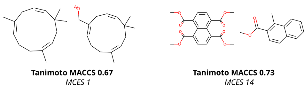
To compare molecular structures, we compute the MCES (Maximum Common Edge Subgraph) of the two molecular structures. Doing so is not new, but comes at the prize that computing a single distance is already an NP-hard problem, see below. Then, why on Earth are we not using Tanimoto coefficients computed from molecular fingerprints, just like everybody else does? Tanimoto coefficients and related fingerprint-based similarity and dissimilarity measures have a massive advantage over all other means of comparing molecular structures: As soon as you have computed the fingerprints of all molecular structures, computing Tanimoto coefficients is blindingly fast. Hence, if you are querying a database, molecular fingerprints are likely the method of choice. We ourselves have been and are heavily relying on molecular fingerprints: CSI:FingerID is predicting molecular fingerprints from MS/MS data, CANOPUS is predicting compound classes from molecular fingerprints, and COSMIC is using Tanimoto coefficients because they are, well, fast. Yet, if you have ever worked with molecular fingerprints and, in particular, Tanimoto coefficients yourself, you must have also noticed their peculiarities, quirks and shortcomings. In fact, from the moment people used Tanimoto coefficients, others have warned about these unexpected and highly undesirable behaviors; an early example is by Flower (1998). On the one hand, a Tanimoto coefficient of below 0.7 can be the result of two compounds with only one hydroxy group added. On the other hand, two highly different compounds, one half the size of the other, may also have a Tanimoto coefficient of 0.7. Look at the two examples below: According to the Tanimoto coefficient, the two structures on the left are less similar than the two on the right. Does that sound right? By the way: The same holds true for any fingerprint-based similarity or dissimilarity measure, and also for any other fingerprint type. These are examples but the problem is universal.
In contrast, the MCES distance is much more intuitive to interpret, as it is the edit distance between molecule graphs and, hence, nicely represents our intuition of chemical reactions. For example, adding an hydroxy group results in an MCES distance of one. Don’t get us wrong: The MCES distance is not perfect, either. First and foremost, the MCES problem is NP-hard; hence, computing a single exact distance between two molecules might take days or weeks. We can happily report that we have “solved” this issue by introducing the myopic MCES distance: We first quickly compute a lower bound on the true distance. If this bound tells us that the true distance is larger than 22, then we would argue that knowing the exact value (maybe 22, maybe 25, maybe 32) is of little help: These two molecules are very, very different, full stop. But if we find that the lower bound only guarantees that the distance is small (say, at most 20) then we use exact computations based on solving an Integer Linear Program. With some more algorithm engineering, we were able to bring down computation time to fractions of a second. And that means that we were able to compute all distances for a set of 20k biomolecular structures, plus several well-known machine learning datasets, in reasonable time and on our limited compute resources. (Sadly, we still do not own a supercomputer.) You will not be able to do all-against-all with a million molecular structures, so if your research requires to do so, you might have to stick with the Tanimoto coefficient, quirky as it is. Yet, we found that subsampling does indeed give us rather reproducible results, see Fig. 7 of the preprint (page 23).
There are other shortcomings of the MCES distance: For example, it is not well-suited to capture the fact that one molecular structure is a substructure of the other. This is unquestioned, but what is also true, is: The MCES distance does not have peculiarities or quirks. The fact that it does not capture substructures, can be readily derived from its definition; this behavior is by design. In case you do not like the absolute MCES distance, because you think that large molecules are treated unfairly, then feel free to normalize it using the size of the molecules. Now that we can (relatively) swiftly compute the myopic MCES distance, we can play around with it.
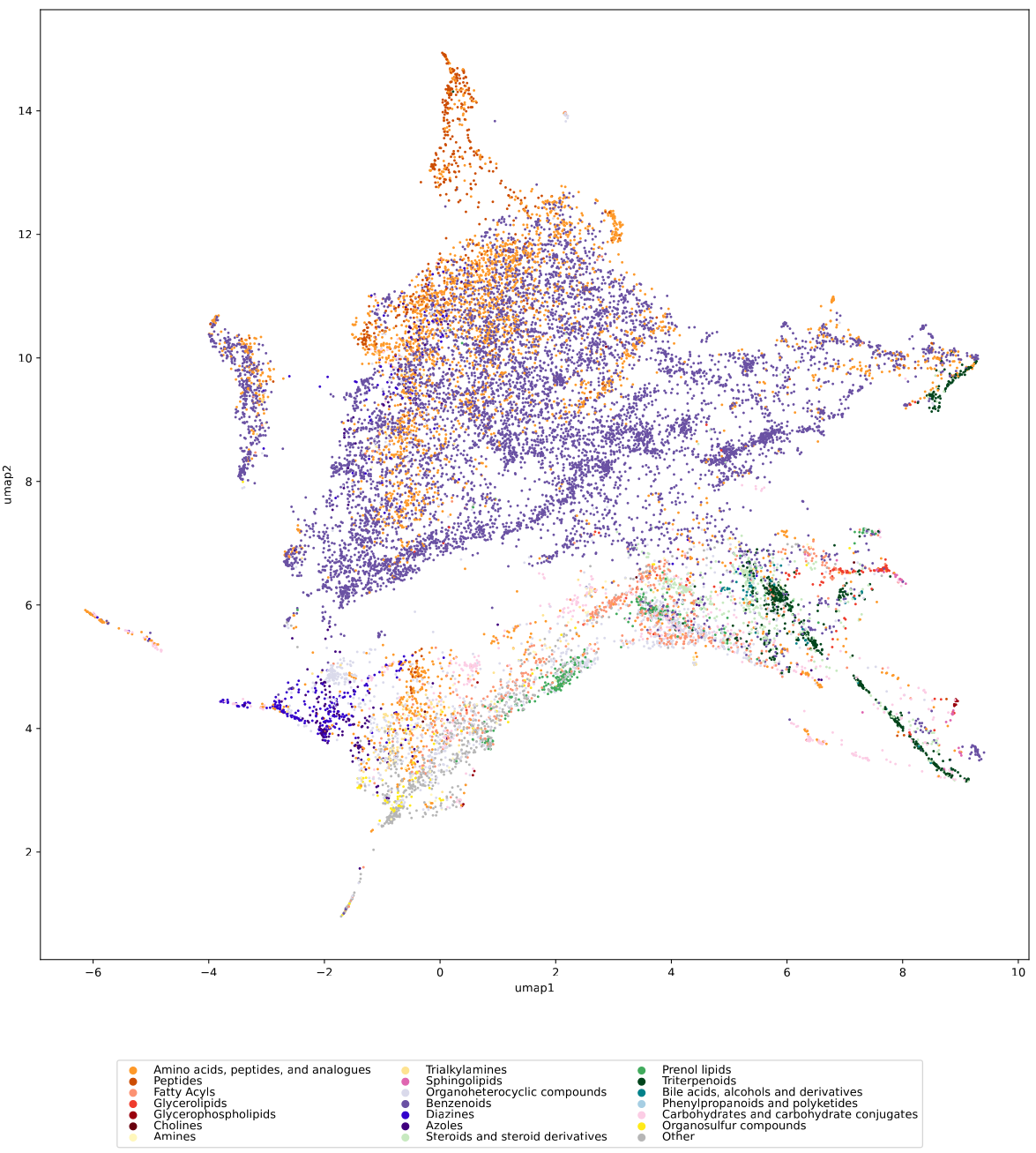
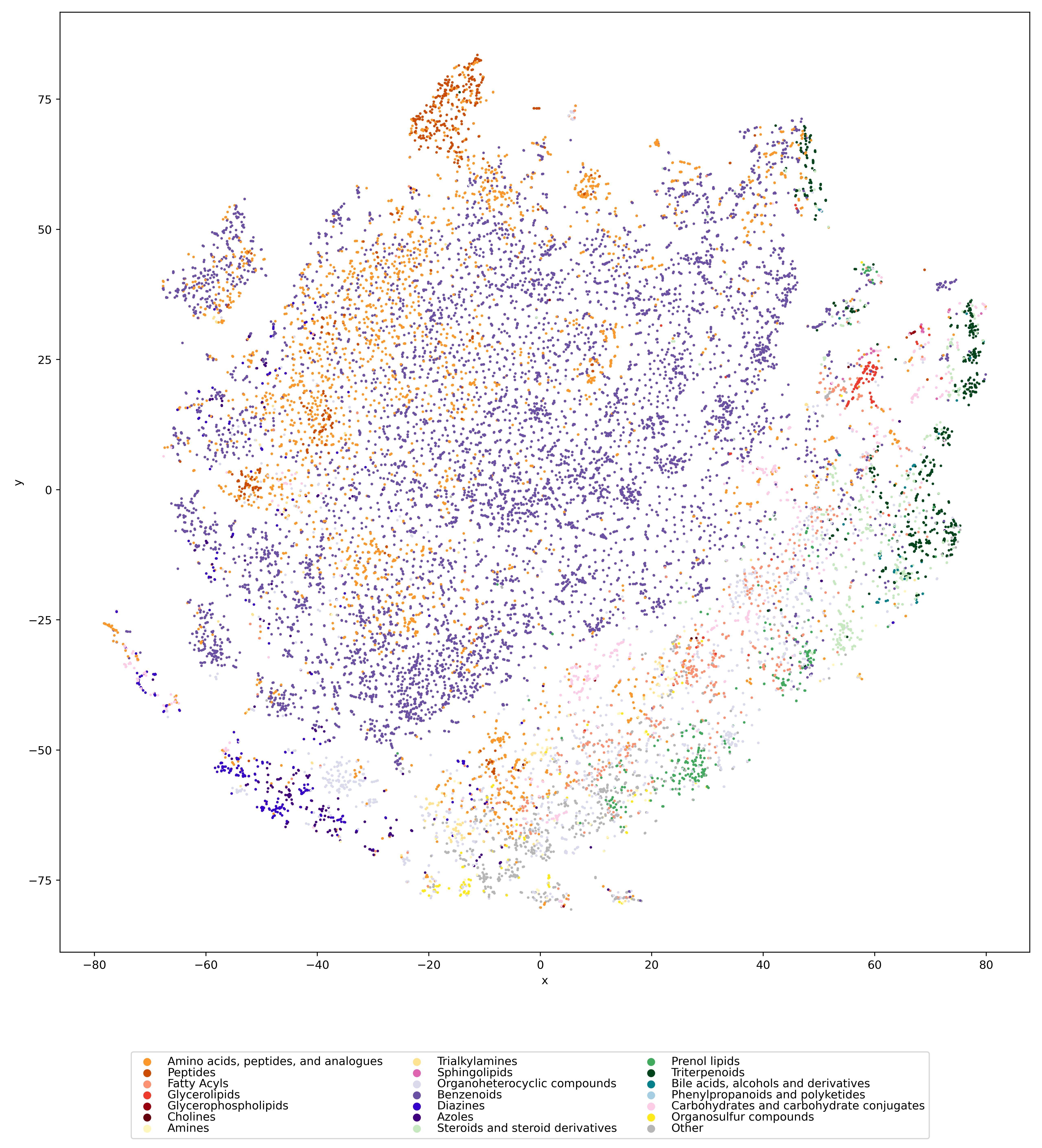
We used UMAP (Uniform manifold approximation and projection) to visualize the universe of biomolecules but, honestly, we don’t care. You prefer t-SNE? Use that! You prefer a tree-based visualization? Use that! See the following comparison (from left to right UMAP, t-SNE and a Minimum Spanning Tree), created in just a few minutes. Or, maybe Topological Data Analysis? Fine, too! All those visualizations have their pros and cons, and one should always keep Pachter’s elephant in the back of one’s brain. But the thing is: We know that the space of molecular structures has an intrinsic structure, and we are merely using the different visualization methods to get a feeling for its intrinsic structure.
Now, one peculiarity of the above UMAP plots must be mentioned here: When comparing different ML training datasets, we re-used the UMAP embedding computed from the biomolecular structures alone (Fig. 3 in the preprint). Yet, UMAP will neatly integrate any new structures into the existing “compound universe” even if those new structures are very, very different from the ones that were used to compute the projection. This is by design of UMAP, it interpolates, all good. So, we were left with two options: Recompute the embedding for every subplot? This would allow us to spot if a dataset contains compounds very different from all biomolecular structures, but would result in a “big mess” and an uneven presentation. Or, should we keep the embedding fixed? This makes a nicer plot but hides “alien compounds”. We went with the second option solely because the overall plot “looks nicer”; in practice, we strongly suggest to also compute a new UMAP embedding.
In the preprint, we discuss two more ways to check whether a training dataset provides uniform coverage of the biological compound space: We examine the compound class distribution, to check whether certain compound classes are “missing” in our training dataset. And finally, we use the Natural Product-likeness score distribution to check for lopsidedness. All of that can give you ideas about the data you are working with. There have been numerous scandals about machine learning models repeating prejudice in the training data; don’t let the distribution of molecules in your training data let you draw conclusions which, at closer inspection, might be lopsided or even wrong.
If you want to compute myopic MCES distances yourself, find the source code here. You will need a cluster node, or proper patience if you do computations on your laptop. All precomputed myopic MCES distances from the preprint can be found here. We may also be able to help you with further computations.