Try out here: 2-step.boeckerlab.uni-jena.de
More about the method: bio.informatik.uni-jena.de/software/2-step/
Friedrich-Schiller-Universität Jena, Fakultät für Mathematik und Informatik
Nils and Andrés will be at the Metabolomics Conference in Buenos Aires, Argentina. Come have a chat and talk some science!
We are part of the second iteration of the Introduction to mass spectrometry techniques and analysis workshop from 4th to 5th of June – hosted by and in the Max Planck Institute for Chemical Ecology! This three-part workshop includes a basic introduction to MS principles and instrumentation, Preprocessing with MZmine as well as Feature annotation using SIRIUS.
Interested researchers outside of Jena (and/or outside the MPI-CE or IMPRS) should contact imprs@ice.mpg.de.
We are at the 7th Central German Meeting on Bioinformatics (also known as Mittelerde) in Halle from 26/03/2026 to 27/03/2026! Sebastian will hold a keynote about small molecule machine learning. Fleming will talk about retention time prediction. Nils, Andres, Leopold and Jonas will have posters to come and look at during the poster session.
On the 24th and 25th of November 2025, our website and our Mattermost instance will be unavailable for multiple hours.
Estimated downtimes are:
Our paper “Barcode-free hit discovery from massive libraries enabled by automated small molecule structure annotation” has finally been published in Nature Communications. This first publication from our joint project with Sebastian Pomplun (Leiden University and Oncode Institute) presents a barcode-free self-encoded library (SEL) platform that enables the screening of over half a million small molecules in a single experiment. Kudos to Sebastian Pomplun and his PhD student Edith van der Nol, and of course to all co-authors!
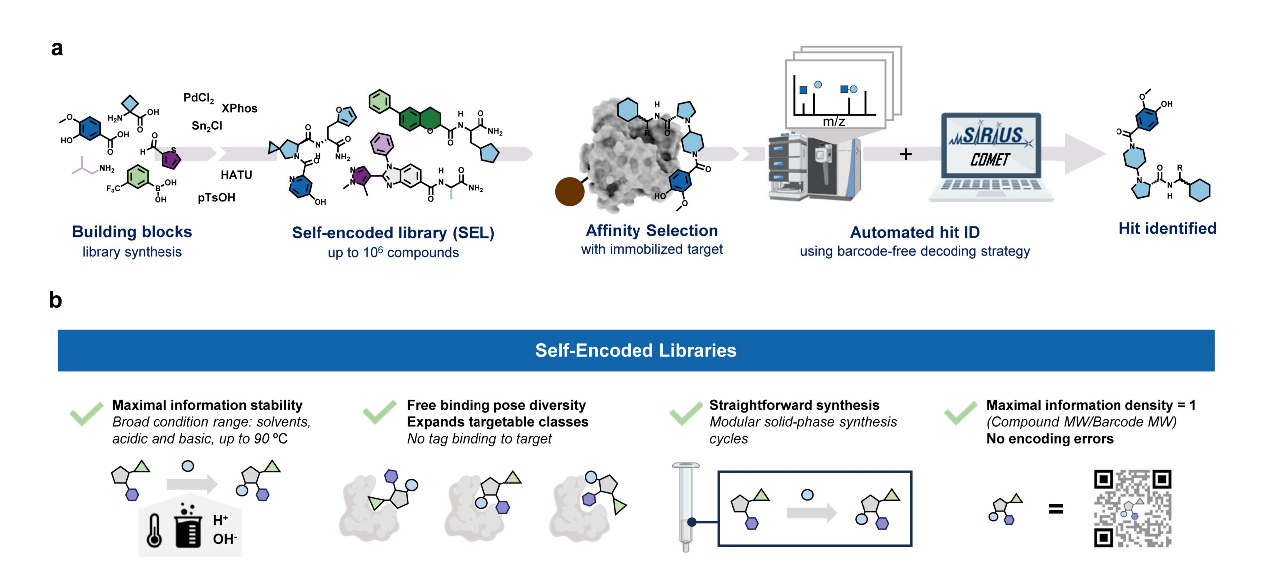
In general, discovering new pharmacologically active molecules that bind to a certain drug target is a tedious process as it requires the screening of very large compound libraries. In contrast to traditional high-throughput methods, affinity selection (AS) represents a powerful approach that allows the rapid screening of millions of molecules in just a single experiment. Here, the compound library is incubated with the receptor of interest, and in a following step, binders are separated from non-binders. This results in a final sample containing ideally only the binders which are called hits.
At this stage of the workflow, we know that this sample represents a subset of our initial screening library, but we do not know which molecules are actually in there. Therefore, the challenge remains in the identification of these hit compounds. This is most commonly done by initially attaching unique DNA barcodes to the molecules of the screening library, which can then be sequenced to identify the isolated hits. However, one of the fundamental drawbacks of these DNA-encoded libraries (DELs) is the potential interference of the attached tag during the affinity selection. This limitation becomes particularly problematic when the target protein has nucleic acid binding sites, making the screening against targets like transcription factors extremely difficult.
Consequently, an approach that does not require any tag while still allowing the simultaneous screening of a vast number of compounds is highly desirable. That is why our screening platform is based on affinity selection-mass spectrometry (AS-MS), which relies solely on MS to identify the selected hit compounds, eliminating the need for any tags. Thus, the name self-encoded libraries (SELs). Since our platform also features the use of split-&-pool libraries, containing potentially millions or even billions of combinatorially synthesized molecules, the monoisotopic mass alone is insufficient for the identification, and tandem mass spectrometry (MS/MS) has to be used instead. Therefore, we present a computational workflow, called COMET, for analyzing the acquired LC-MS/MS data and enabling the identification of the isolated hit compounds. Although the final AS sample contains only up to a few hundreds compounds, we observed that the corresponding LC-MS/MS data mainly contained features resulting from background noise, which usually lead to a large number of false-positive annotated compounds. We therefore implemented a filter into COMET that removes all features that do not match a genuine library molecule, either due to a non-matching precursor mass or fragmentation pattern.
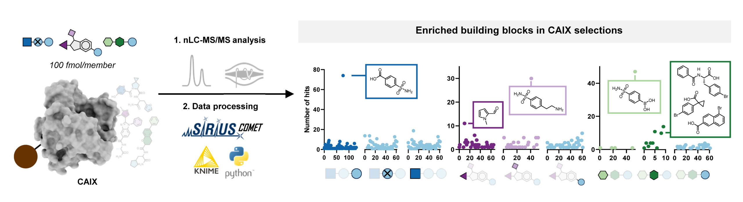
With this workflow in hand, Edith synthesized three combinatorial molecule libraries containing up to 750,000 compounds and incubated them separately with carbonic anhydrase IX (CAIX), a target typically used to benchmark novel DNA-encoded libraries. All three AS-MS experiments resulted in the identification of hit compounds containing a sulfonamide building block, which aligns well with the literature about known CAIX binders. Subsequent validation confirmed these hits’ binding affinity to CAIX, demonstrating the effectiveness of our screening platform.
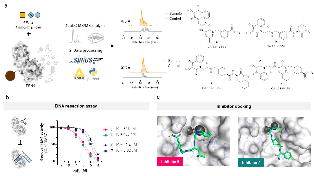
But this represents more or less only a sanity check and does not clearly show the advantage of our SEL platform compared to DELs. So, we chose a target protein which is beyond the scope of DELs: flap endonuclease 1 (FEN1), a DNA-processing enzyme essential for replication and repair, and over-expressed in multiple cancer types. For this challenging target, we synthesized a new, more focused library comprising 4,000 members after determining that our previous libraries were insufficient for clear hit identification. This approach successfully yielded four hits, all of which demonstrated inhibitory activity against FEN1.
All in all, our SEL-COMET workflow represents a rapid, barcode-free screening approach for early drug discovery, and we hope that this approach will be widely adopted in both academic and industrial research settings.
A quick reminder: The PhD and postdoc positions within the ERC project BindingShadows are still open!
We’ve just moved into a brand-new building, and during the transition our servers and website were occasionally down, meaning we might not have received some applications. So once again: if you’re skilled in bioinformatics and/or machine learning, and you’re excited about developing innovative computational methods for analyzing small molecule mass spec data, please apply! The project is based in Jena, Germany, and will run for five years. At least two postdoctoral and two PhD positions are available. For questions, feel free to contact us — and please share this with anyone who might be interested. Thank you!
We moved! After several weeks of home office, we finally moved into our brand-new building!
Apologies for the occasional downtime of our servers and website over the past two months. Everything is back up and should run smoothly from now on!


On the 20th and 21st of October 2025, our website and our Mattermost instance will not be available. This is due to stress testing of the compute infrastructure at our new building. The SIRIUS services like CSI:FingerID will stay up and running. We hope to be back at full operation on Wednesday and should stay up from then on!
After three weeks, our web server (and many other things) are back online. We made sure that CSI:FingerID etc are up and running, but somehow forgot that there is more than that. Sorry in case this caused any troubles.
Im kommenden Wintersemester 2025/2026 wird wieder das Modul Bioinformatische Methoden in der Genomforschung angeboten. Im Sommersemester 2026 wird dann wieder das Modul Sequenzanalyse zu hören sein.
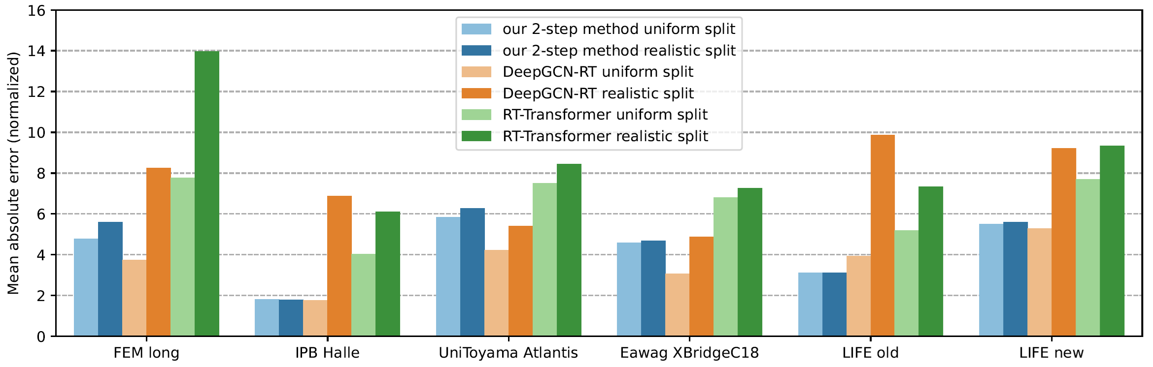
We just solved a problem that I never wanted to solve: That is, transferable retention time prediction of small molecules. They say that the best king is someone who does not want to be king; so maybe, the best problem solver is someone who does not want to solve the problem? Not sure about that. (My analogies have been quite monarchist lately; we are watching too much The Crown.)
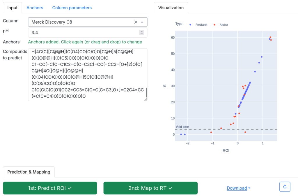
What is transferable retention time prediction? Let’s assume you tell me some details about your chromatographic setup. We are talking about liquid, reversed-phase chromatography. You tell me what column you use, what gradient, what pH, maybe what temperature. Then, you say “3-Ketocholanic acid” and I say, “6.89 min”. You say “Dibutyl phthalate”, I say “7.39 min”. That’s it, folks. If you think that is not possible: Those are real-world examples from a biological dataset. The true (experimentally measured) retention times where 6.65 min and 7.41 min.
Now, you might say, “but how many authentic standards were measured on the same chromatographic setup so that you could do your predictions”? Because that is how retention time prediction works, right? You need authentic standards measured on the same system so that you can do predictions, right? Not for transferable retention time prediction. For our method, the answer to the above question is zero, at least in general. For the above real-world example, the answer is 19. Nineteen. In detail, 19 NAPS (N-Alkylpyridinium 3-sulfonate) molecules were measured in an independent run. Those standards were helpful, but we could have done without them. If you know a bit about retention time prediction: There was no fine-tuning of some machine learning model on the target dataset. No, sir.
Now comes the cool part: Our method for retention time prediction already performs better than any other method for retention time prediction. The performance is almost as good as that of best-in-class methods if we do a random (uniform) split of the data on the target system. Yet, we all know (or, we all should know) that uniform splitting of small molecules is not a smart idea; it results in massively overestimating the power of machine learning models. Now, our model is not trained (fine-tuned) on data from the target system. Effect: Our method works basically equally well for any splitting of the target dataset. And, we already outperform the best-in-class method.
Why am I telling you that? I mean, besides showing off? (I sincerely hope that you share my somewhat twisted humor.) And, why did I say “already” above? Thing is, retention time prediction is dead, and you might not want to ruin your PhD student’s career by letting him/her try to develop yet another machine learning model for retention time prediction. But now, there is a new, much cooler task for you and/or your PhD student!
Now, how does the 2-step method work? The answer is: We do not try to predict retention times, because that is impossible. Instead, we train a machine learning model that predicts a retention order index. A retention order index (ROI) is simply a real-valued number, such as 0.123 or 99999. The model somehow integrates the chromatographic conditions, such as the used column and the mobile phase. Given two compounds A and B from some dataset (experiment) where A elutes before B, we ask the model to predict two number x (for compound A) and y (for compound B) such that x < y holds. If we have an arbitrary chromatographic setup, we use the predicted ROIs of compounds to decide in which order the compounds elute in the experiment. And that is already the end of the machine learning part. But I promised you transferable retention time, and now we are stuck with some lousy ROI? Thing is, we found that you can easily map ROIs to retention times. All you need is a low-degree polynomial, degree two was doing the trick for us. No fancy machine learning needed, good old curve fitting and median regression will do the trick. To establish the mapping, you need a few compounds where you know both the (predicted) ROI and the (measured) retention time. These may be authentic standards, such as the 19 NAPS molecules mentioned above. If you do not have standards, you can also use high-confidence spectral library hits. This can be an in-house library, but a public library such as MassBank will also work. Concentrate on the 30 best hits (cosine above 0.85, and 6+ matching peaks); even if half of these annotations are wrong, you may construct the mapping with almost no error. And voila, you can now predict retention times for all compounds, for exactly this chromatographic setup! Feed the compound into the ROI model, predict a ROI, map the ROI to a retention time, done. Read our preprint to learn all the details.
At this stage, you may want to stop reading, because the rest is gibberish; unimportant “historical” facts. But maybe, it is interesting; in fact, I found it somewhat funny. I mentioned above that I never wanted to work on retention time prediction. I would have loved if somebody else would have solved the problem, because I thought my group should stick with the computational analysis of mass spectrometry data from small molecules. (We are rather successful doing that.) But for a very long time, there was little progress. Yes, models got better using transfer learning (pretrain/fine-tune paradigm), DNNs and transformers; but that was neither particularly surprising nor particularly useful. Not surprising because it is an out-of-the-textbook application of transfer learning; not particularly useful because you still needed training data from the target system to make a single prediction. How should we ever integrate these models with CSI:FingerID?
In 2016, Eric Bach was doing his Master thesis and later, his PhD studies on the subject, under the supervision of Juho Rousu at Aalto University. At some stage, the three of us came up with the idea to consider retention order instead of retention times: Times were varying all over the place, but retention order seemed to be easier to handle. Initially, I thought that combinatorial optimization was the way to go, but I was wrong. Credit to whom credit is due: Juho had the great idea to predict retention oder instead of retention time. For that, Eric used a Ranking Support Vector Machine (RankSVM); this will be important later. This idea resulted in a paper at ECCB 2018 (machine learning and bioinformatics are all about conference publications) on how to predict retention order, and how doing so can (very slightly) improve small molecule annotation using MS/MS. (Eric and Juho wrote two more papers on the subject.)
The fact that Eric was using a RankSVM had an interesting consequence: The RankSVM is trained on pairs of compounds, but what it is actually predicting is a single real-valued number, for a given compound structure. For two compounds, we then compare the two predicted numbers; the smaller number tells you the compound that is eluting first. In fact, the machine learning field of learning-to-rank does basically the same, in order to decide which website best fits with your Google DuckDuckGo query. I must say that back then, I did not like this approach at all; it struck me as overly complicated. But after digesting it for some time, I had an idea: What if we do not use ROIs to decide which compounds elutes first? What if we instead map these ROIs to retention times, using non-linear regression? Unfortunately, I never got Eric interested to go into this direction. And I tried; yes I tried.
About seven years ago, Michael Witting and I rather reluctantly decided to jointly go after the problem. (I would not dare to go after a problem that requires massive chemical intuition without an expert; if you are a chemist, I hope you feel the same about applying machine learning.) We had my crazy idea of mapping ROIs to retention times, and a few backup plans in case this would fail. We had two unsuccessful attempts to secure funding from the Deutsche Forschungsgemeinschaft. My favorite sentence from the second round rejection is, “this project should have been supported in the previous round as the timing would have been better”; we all remember how the field of retention time prediction dramatically changed from 2018 to 2019…? But as they say, it is the timing, stupid! We finally secured funding in May 2019; and I could write, “and the rest is history”. But alas, no. Because the first thing we had to learn was that there was no (more precisely, not enough) training data. Jan Stanstrup had done a wonderful but painstaking job to manually collect datasets “from the literature” for his PredRet method. Yet, a lot of metadata were missing (these data are not required for PredRet, we must not complain) and we had to dig into the literature and data to close those gaps. Also, we clearly needed more data to train a machine learning model. With this, our hunt for more data began, which we partly scraped from publications, partly measured on our own; kudos go to Eva Harrieder! This took much, much longer than we would ever have expected, and resulted in the release of RepoRT in 2023. Well, after that, it is the usual. It works, it doesn’t work, maybe it works; next, it is all bad again; the other methods are so much better; the other methods have memory leakage; now, we have memory leakage; and finally, success. Phew… And here it is.
What about HILIC? I have no idea; but I can tell you that it is substantially more complicated. In fact, there currently is not even a description of columns comparable to HSM and Tanaka for RP. Maybe, somebody wants to get something started? Also, HILIC columns are much more diverse than RP columns, meaning that we need more training data (currently, we have less) and a better way to describe the column than for RP. But hey, start now so that it is ready in 10 years; worked for us!
References
Now, that number deserves a celebration: Our web services have served a billion queries! In detail, the CSI:FingerID web service processed 759 million queries, the CANOPUS web service 228 million, and MSNovelist has 17 million queries. During the last 12 months, 3816 users have processed their data using our web services. Excellent!
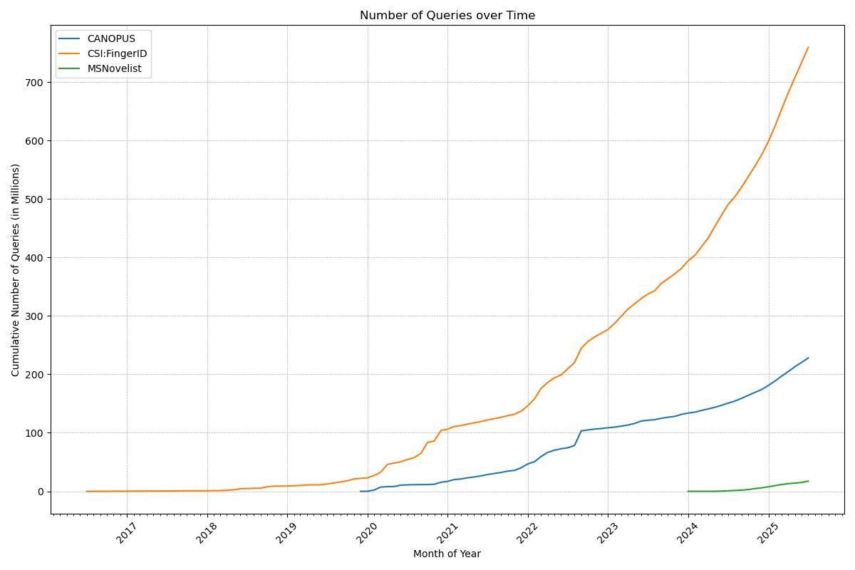
Remember when Gangnam Style was the first video on YouTube to hit 1 billion views? That was a big thing in December 2012; we do not expect the same amount of media coverage for our first billion, though. 😉 Indeed, one billion is a big number, and it is really hard to grasp it: See this beautiful video by Tom Scott to “understand” the difference between a million and a billion.
Anyways, many thanks to the team (mainly Markus Fleischauer) who make this possible, and who ensure that everything is running so smoothly! It should not be a surprise that processing 1.18 million queries per day (on average!), is a highly non-trivial undertaking. Auto-scalable, self-healing compute infrastructure and highly optimized database infrastructure are key ingredients for keeping small molecule annotations flowing smoothly to our global community.
PS. The one billion also cover the queries processed by the Bright Giant and their servers, who are offering these services to companies. One counter to rule them all…
Excellent news: Sebastian will receive an ERC Advanced Grant from the European Research Council!
In the project BindingShadows, we will develop machine learning models that predict whether some query molecule has a particular bioactivity (say, toxicity) or is binding to a certain protein, where the only information we have about the query molecule is its tandem mass spectrum. The clue is: The model is supposed to do that when the identity and structure of the molecule is not known; not known to us, not known to the person that measured the data, not known to mankind (aka novel compounds).
Clearly, we will not do that for one bioactivity or one protein, but for all of them in parallel. Evolution has, through variation and selection, optimized the structure of small molecules for tasks such as communication and warfare, and the pool of natural products is enriched with bioactive compounds. Our project will try to harvest this information.
Sounds interesting? Looking for a job? Stay tuned, as we will shortly start searching for PhD and postdoc candidates!
Markus and Jonas will contribute to the summer school with a workshop about SIRIUS. For all interested, it takes place 18. to 22. August 2025 in Copenhagen, Denmark. We hope to meet many of you there!
Im kommenden Semester wird statt Sequenzanalyse das Modul Algorithmische Phylogenetik angeboten. Sequenzanalyse wird dann wieder im SoSe 2026 zu hören sein.
We’re excited to announce the latest version of SIRIUS designed to improve your small molecule analysis workflow with a refreshed interface, streamlined processes, and several important fixes that ensure smoother performance and better data handling.
? New Color Scheme: A consistent and intuitive look throughout the entire identification process.
⚡ Streamlined Workflows: Tools are now automatically activated/deactivated to comply with SIRIUS workflow principles. You can also easily save and reload computation settings with our new preset function.
? Welcome Page Redesign: Get a quick overview of your account, connection details, and helpful resources to make the most of SIRIUS.
? Improved Result Views: Numerous enhancements and fixes across result views for a smoother analysis experience.
Our preprint Times are changing but order matters: Transferable prediction of small molecule liquid chromatography retention times is finally available on chemRxiv! Congratulations to Fleming and all authors.
In short, we show that prediction of retention times is a somewhat ill-posed problem, as retention times vary substantially even for nominally identical condition. Next, we show that retention order is much better preserved; but even retention order changes when the chromatographic conditions (column, mobile phase, temperature) vary. Third, we show that we can predict a retention order index (ROI) based on the compound structure and the chromatographic conditions. And finally, we show that one can easily map ROIs to retention times, even for target datasets that the machine learning model has never seen during training. Even for chromatographic conditions (column, pH) that are not present in the training data. Even for “novel compounds” that were not in the training data. Even if all of those restrictions hit us simultaneously.
In principle, this means that transferable retention time prediction (for novel compounds and novel chromatographic conditions) is “solved” for reversed-phase chromatography. There definitely is room for improvement, but that mainly requires more training data, not better methods. For that, we need your help: We need you, the experimentalists, to provide your reference LC-MS datasets. It does not matter what compounds are in there, it does not matter what chromatographic setup you used; as long as it is references data measured from standards (meaning that you know exactly each compound in the dataset), and as long as you tell us the minimum metadata, this will improve prediction quality.
You can post your data wherever you like, but you can also upload them to RepoRT so that in the future, scientists from machine learning can easily access them. We now provide a web app that makes uploading really simple. If you are truly interested in retention time prediction, then this should be well-invested 30 min.
Jonas will give a lecture on SIRIUS at the IMPRS course “Introduction to mass spectrometry techniques and analysis” (2-4 December) in the Max Planck Institute for Chemical Ecology.